OPERATIONS MANAGEMENT

ECONOMIC ORDER QUANTITY MODEL

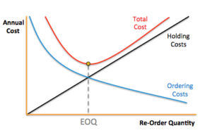
The inventory problems in which demand is assume to be fixed and completely predetermined are usually referred to as the Economic Order Quantity (EOQ). By the order quantity, we mean the quantity produced or procured during one production cycle. When the size of order increases the ordering costs will decrease whereas the inventory carrying cost will increase. Thus in the production process there are two opposite costs; one encourages the increase in the order size and other discourages the order size. EOQ is that size of order which minimizes total annual costs of carrying inventory and cost of ordering.

ASSUMPTIONS:

Demand for the inventory is deterministic i.e. it is known with certainty.

Demand rate is constant and known beforehand.

All orders are placed in single lot.

No stock out shortages or back orders are allowed.

No quantity discount is allowed. This purchase cost per unit is fixed.

Lead time is constant and it is independent of demand.

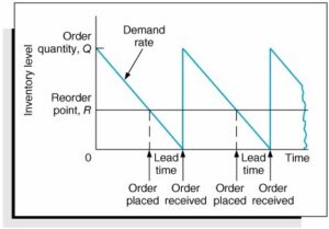
Safety Stock (q_o) is the minimum limit of inventory which must be in stores at any time.

Lead Time between when an order is placed and when the order is received.

D= Annual demand of inventory items ([frac up=”units” down=”year”])

Q= Quantity to be ordered at each point ([frac up=”units” down=”order”])

d = Demand or consumption rate

N= Number of orders in a year ([frac up=”order” down=”year”])

T= Time gap between two successive orders ([frac up=”year” down=”order”])

Example:

D= 54000 [frac up=”units” down=”year”]

Q= 9000 [frac up=”units” down=”order”]

therefore, N = [frac up=”D” down=”Q”] = 54000/9000 = 6 [frac up=”order” down=”year”]

C= Cost of purchasing 1 unit of inventory item ([frac up=”Rs” down=”unit”])

C_o= Cost of placing 1 order ([frac up=”Rs” down=”order”])

C_h= Cost of holding 1 unit inventory for 1 complete year

Total Annual Cost (TAC) = Purchase Cost (PC) + Ordering Cost (OC) + Holding Cost (HC)

Purchase Cost (PC) = D x C

Ordering Cost (OC) = N x Co = [frac up=”D” down=”Q”] x C_o

Holding Cost (HC) for period T = [frac up=”Q” down=”2″]. C_h. T

Average inventory carried during the year =

Q + [frac up=”0″ down=”2″] = [frac up=”Q” down=”2″] [ Inventory level is uniformly decreasing from Q to zero]

Annual Handling Cost (HC) = [frac up=”Q” down=”2″] . C_h. T.N

= [frac up=”Q” down=”2″] . C_h (T.N =1)

Total Annual Cost (TAC) = D x C + [frac up=”D” down=”Q”] x Co + [frac up=”Q” down=”2″] x C_h

The Total Variable Cost or Total Inventory Cost = OC + HC

Total Inventory Cost (TIC) = [frac up=”D” down=”Q”]. C_o + [frac up=”Q” down=”2″] . C_h

Total Annual Cost (TAC) = Total Inventory Cost (TIC) + Direct Cost (DC)

At EOQ (Q*), OC = HC

[frac up=”D” down=”Q*”] x C_o = [frac up=”Q*” down=”2″] x C_h

Q* = √(2.D.[frac up=”C_o” down=”C_h“] )

TIC* = [frac up=”D” down=”Q*”] x C_o + [frac up=”Q*” down=”2″] x C_h (TIC* = Total Inventory Cost at EOQ)

but [frac up=”D” down=”Q*”] x C_o = [frac up=”Q*” down=”2″] x C_h

TIC* = 2 x [frac up=”Q*” down=”2″] x C_h = Q*

TIC*= √(2.D.Co.Ch)

ABC ANALYSIS

ABC is Always Better Control or Alphabetical Approach.

ABC analysis divides the inventory into three groups in terms of percentage of number of items and percentage of total value.

It is based on Pareto analysis.

A TYPE INVENTORY:

These are high value, low volume type of inventories. This means that their annual consumption is very less but these are very costly items.

These items need accurate, careful handling and storage under tight control. Such items should be thought of in advance and purchased well in time. A detailed record or receipt should be kept and proper handling of facilities should be provided for them.

Such items being costly are purchased in small quantity often and just before the use. This, off course increases the procurement cost and involves little risk of non-availability. However, inventory holding cost decreases and problems of storage and caretaking are minimized.

C TYPE INVENTORY:

These are low value, high volume type of inventories. This means that their annual consumption is high but these are less costly items.

Majority of items (70%) constitute only a minor fraction of total annual monetary consumption (10%).

B TYPE INVENTORY:

These are middle level items which do not requires detailed and close control as A items but hey need more attention and control than C items.

These items represents 20% of the total quantity of items and 15% to 20% of the total expenditure on items.

Category	Percentage of item	Percentage of value
A	10%	70%
B	20%	20%
C	70%	10%

A ITEMS – CONTROL POLICIES:

A items are high valued items hence they should be ordered more frequently but in small quantities in order to reduce capital locked up at any time.

The future requirement must be planned in advance so that the required quantities arrive a little before they are required for consumption.

Purchase and stock control of A items should be looked into by the top executives in purchasing department.

Ordering quantities, reorder point and minimum stock level should be revised more frequently.

C ITEMS – CONTROL POLICIES:

These are low valued items therefore the safety stock of such items should be liberal.

Annual or six monthly orders should be placed to reduce paper work and ordering cost and to get advantage of quantity discount for large orders.

In case of these items only routine check is required.

B ITEMS – CONTROL POLICIES:

Policies for B items in general are between those for A & C.

Order for those items must be placed less frequently.

Safety stock should be medium (3 months or less).

Subjected to moderate control.

STEPS IN ABC ANALYSIS:

Calculate the annual usage in units for each items.

Calculate annual usage of each item in terms of rupees.

Rank the items from highest annual usage in rupees to lowest annual usage in rupees.

Compute total rupee.

Find the percentage of high, medium and low valued items in terms of total value of items.

MATERIALS MANAGEMENT- Economic order quantity & ABC Analysis